
Causal Set Theory (CST) is one of the current serious attempts at creating a discrete model of the fine level structure of spacetime. It relies on a small number of basic assumptions. It is accessible to non-experts. The plausibility of some of the effects of special relativity can be seen quite simply without any mathematics. In this post I am going to show in diagrams how this happens. You won’t need any technical knowledge here, you won’t need to know anything about special relativity, and you won’t have to look at a single equation. (For those interested, I’ll quarantine some equations and technical details in sections in a coloured font, but there is no need to look at these if you don’t want to.)
Currently there is a lot of early stage theoretical investigation going on in CST. Some of it is looking into special relativity. This post will show the sort of ideas that are being thrown around. In particular I’ll be trying to show intuitively how time dilation, length contraction and increase in mass are quite natural in CST.
It is precisely the discrete nature of CST that allows this more intuitive understanding of special relativity. Keeping track of a finite number of points is much simpler than keeping track of an infinite number of them. Basically, CST lends itself to visual explanation much better.
So without any nasty infinities to bother us, let’s go…
First, the diagrams. They represent one dimension of space going from left to right, and the one dimension of time going upwards to the future. Although our universe has 3 dimensions of space, special relativity has the convenient property that it can be explained quite well in one spatial dimension. Here is an example at the macroscopic level:
Figure 1: A typical bit of macroscopic spacetime with one spatial dimension.
Object A is stationary in space, it just flows through time. B has a constant velocity from right to left. The moving dotted line are the simultaneous points in the one dimensional space (spoiler: as far as A is concerned). Traditionally these discussions talk about trains moving on a track, since they approximate one dimension very well. A and B can be thought of as train carriages along a long straight track.
Now we’ll dive down to where the causal sets live and see what they look like. We’ll go down past the size of atoms (10-10metres or 1/10000000000 of a metre), past the nucleus of an atom (10-15 metres), and we’ll keep going much much further down to what is widely held to be rock bottom at around 10-35 metres. This is known as the Planck scale and it’s where physics as we know it breaks down.
Here, in CST, there is no spacetime continuum. There are dots and there are joins between dots. Each line has an inherent direction, which will be the direction of causality. CST says that our universe is one really big causal set.
Figure 2 shows randomly placed dots. All the dots are joined to each other (I’ll be using the term line and join interchangeably). I have not shown the joins’ directions as the diagram is confusing enough. There are also some random dots outside the diagram (with the same density of dots), extending another half the diagram width to the right and left, and another half the diagram height above and below. The visible dots are also joined to all the dots off the screen. If I kept extending to more off-screen dots, the diagram would become black.
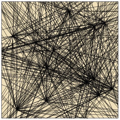
Figure 2: A bit of a causal set, directions not shown.
Because the causal set is only dots and directional joins, this means that the sepia coloured background is not part of the set and so is not part of our universe. It is only there because we live in a seemingly continuous universe at the macroscopic level and your computer screen is effectively two dimensional and continuous. This is quite convenient because it means we can show the dots and joins diagrammatically in an intuitive way, but it is essential to understand that only the joins and dots exist.
In this post we’re going to visualise information as moving from dots, along the lines, in their causal direction, to adjacent dots, and then impacting on the information in the adjacent dot. In figure 2 all dots are adjacent because all are connected to every other dot. But information doesn’t really move along the line. That’s just a convenient notion to help us visualise causal sets. There is actually no notion of distance between dots at this stage. When we think of information moving from dot A to dot B, what’s really happening is that dot A’s information is causally affecting dot B’s information. The lines, however, are very convenient for visualisation.
The dots can be called events and I will use the two terms interchangeably. In normal language an event is something that happens, but in physics it is a location, in space and time. For example, the centre of train carriage B at precisely 12:45 PM is an event. These dots in the diagrams are locations in space and time.
Here is the first CST rule:
Rule 1: Information can only move in an upwards direction.
If we now interpret figure 2 in the same way as figure 1, that is with space going across and time going upwards, then this is the same as saying causality can only operate in the direction of time. An event in the future cannot affect an event in the past, but events in the past can affect events in the future. Think of each line in figure 2 as having an arrowhead at the higher end to indicate direction.
Here’s the next rule:
Rule 2: Information moves slower than the speed of light.
Speed, or velocity, is space covered per time. A nearly vertical line has low velocity, a nearly horizontal line has high velocity. If we choose the vertical time scale and the horizontal spatial scale specifically so that a 45° line corresponds to moving at the speed of light, then that means lines must have slope greater than 45°. So let’s remove all the faster-than-light lines from figure 2:
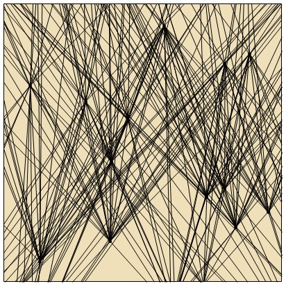
Figure 3: The same bit with only lines >45° shown. All arrowheads would be at the higher end of each line.
Special relativity was derived from one experimentally observed fact, that light always travels at the same speed (in a vacuum), which we’ll call c, which is about 300,000 kilometres per second. That’s always at the same speed relative to you. Even if you’re travelling at half the speed of light yourself, light still travels past you at speed c relative to you. This makes no sense. For it to be true, something has to be seriously wrong with our ‘normal’ understanding of physics. And it is.
The law that light always travels at the same speed is here replaced by the weaker Rule 2. Note that the extent of the CST model I’m using here does not incorporate objects that can move at the speed of light, it is not sufficiently detailed to do that.
More technically: Embedding
These dots are randomly sprinkled. Then we insert all the joins that are greater than 45° and set causality going upwards. Then we in principle discard the background because it’s not part of the universe. We do it in this order purely for convenience. We want a causal set that embeds into a normal flat Euclidean space. Embeddable when applied to an arbitrary causal set means that the set (dots and lines only) has the property that it can be pushed and pulled into a shape that fits into a Euclidean space, with all joins over 45° and pointing upwards. Rather than start with a causal set and see if it is possible to do this, we do it the other way around by random sprinkling. Random sprinkling is not necessarily a real part of the construction of our universe. We want our causal set to be embeddable because then at macroscopic levels we’d expect to find an (apparently continuous) Euclidean space emerge.
Almost all causal sets are not embeddable, for example three dots all joined with directions a to b, b to c and c to a won’t work. So, when we talk about lines being over 45° we are not relying on the existence of the background, rather we’re relying on the dots and joins being embeddable.
Distance in a Causal Set
We’ll now look at what constitutes distance between dots. To visually simplify I’ll now remove the lines that involve dots that are out of view:
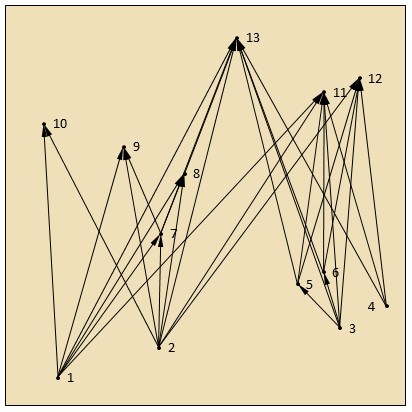
Figure 4: The same bit with only lines >45°, dots out of view removed, and causality direction shown.
In figure 4, dot 2 causally affects 8 because there is a line linking 2 to 8, but 2 does not causally affect 5 as there is no line joining them. Information can move from 2 to 8 in one step, or in two steps by going via 7. For two causally connected dots there will generally be lots of different paths, of a differing number of steps, and there will always be a single step path.
So how do we define distance between two dots? It is going to depend in some way on the number of steps in a collection of different length paths. The answer is a third rule of CST:
Rule 3: The distance between two dots is the number of steps of the longest possible path between the two dots.
So the distance between 2 and 13 is three, by going via 7 and 8.
You can think of the distance in terms of a playing piece moving in a board game, or if you prefer, as discrete steps in the evolution of a discrete wave function.
We can see that movement along most lines has a vertical and a horizontal component, corresponding to movement in time and movement in space respectively. But from the perspective of the travelling bits of information, they only know they are moving from one dot to a causally downstream dot (which means upwards in a diagram). They always see each line as simply forward. They have no concept of distinguishing between movement in space and movement in time. There is only forward. The number of steps taken is the number of causal evolutions that happen. If you accept that the flow of time is simply the effecting of causality, then the number of steps is the amount of elapsed time, from the point of view of the travelling information.
To put it simply, if the information carried a watch, each step would be one tick of the watch. Each tick causes the information to evolve and hence experience time. This notion of the amount of time experienced by an object is referred to as proper time.
Time Dilation
Now let’s have a look at a larger bit of spacetime.
Figure 5: Information passing through lines of maximum distance from A to B.
In figure 5 you can see all the lines of maximum length going from dot A (the bottom corner of the rectangle of dashed lines) to dot B (the top corner of the rectangle). Any path from A to B, maximum length or otherwise, will always be contained within this “45° rectangle” constructed from the four lines passing through A and B at 45°. Any path from A to B going outside the rectangle would at some stage need a line of <45°, violating Rule 2.
The maximum path length turns out to be 8 between A and B and so we’ll consider the elapsed time for something travelling from A to B as 8.
In figure 5 the dots are placed randomly, except for a bit of a fudge I’ve done. Although it was nearly impossible to pick it out, there is another 45° rectangle where I’ve placed exactly the same causal set as that contained in the A to B rectangle. Here it is, C to D:
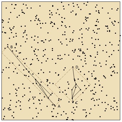
Figure 6: Same patch with identical area highlighted.
They have an identical pattern of causal connections, but are embedded somehow differently. Since the background is not part of spacetime, they are in all regards identical pieces of spacetime. Clearly then there is some choice of how we place a causal structure into a diagram. The CD rectangle is actually a square and D is directly above C. Thus the journey from C to D is considered stationary in space. The AB rectangle is obtained by stretching the CD rectangle to 3 times the length in the bottom-right to top-left direction, and squashing to one third the length in the bottom-left to top-right direction. This turns out to be equivalent to the journey from A to B being at 80% of the speed of light (horizontal difference divided by vertical difference) or .8c.
Both rectangles have the same visual area. Stretching and/or squashing along these two 45° angled directions is the only way to guarantee that lines connecting dots always remain at an angle greater than 45°, and dots that aren’t connected never achieve an angle greater than 45°. If you also want to maintain a uniform density of dots everywhere, then this stretching must be uniform everywhere and the amount of stretching in one direction must be the same as the shrinking in the other direction.
So let’s stretch the whole of figure 6 in this way to try and get AB to look like CD:
Figure 7: Same patch, with changing viewpoint.
At the start of the animation, C to D is stationary while A to B is travelling at .8c to the left. By the end of the animation A to B is stationary while C to D is travelling at .8c to the right. This stretching shows how every moving object can be considered stationary: you only have to stretch the diagram until an object’s movement in spacetime looks vertical (ie stationary). These are referred to as frames of reference and figure 7 starts in CD’s frame of reference and ends in AB’s frame of reference. Moving objects will all feel as though they are stationary, they all see things from the perspective of their own frame of reference.
At the end of the animation, the AB rectangle is visually identical to CD at the start. The journeys from A to B and from C to D are identical. Both take 8 units of proper time. Eight ticks of their watches.
In CD’s frame of reference, as shown in figure 6, when the information going from C to D looks across at the information travelling from A to B, it sees A to B’s wristwatch ticking more slowly. A to B has to travel a much larger vertical distance for the same number of ticks, by a factor of 5/3 in this case. This is the relativistic effect of time dilation. And the effect is symmetric: at the end of the animation in figure 7, when it is in A to B’s frame of reference, A to B looks across to see C to D’s wristwatch ticking slowly. Both see that time has slowed down in the other object.
An assumption should now be made explicit: if an object is stationary in a diagram then it views events along a horizontal line as being simultaneous. I’m not addressing why this is so in this post. It requires a bit of work to even define what simultaneous really means. I’ll just say it’s intuitive and leave it at that for now. So a statement like “C to D looks over at A to B…” really means “C to D looks over at simultaneous events of A to B…”. For objects not stationary in a diagram, their perceived line of simultaneity is very much not horizontal.
More technically:
Quite straightforward Euclidean geometry of the two rectangles shows that when, say, C to D is in the stationary configuration, A to B is taller by a factor of
where v is 
and so


Length Contraction
In figure 7, the rectangles not only stretch out vertically, but they also shrink horizontally. This horizontal shrinking is relativistic length contraction. By stretching the rectangle more and more its horizontal width can be made as small as you like. But figure 7 doesn’t give much precision on how much the length contraction is. Figure 8 shows the effect more precisely, with stretching by 3 and squashing to 1/3 again.
Figure 8: Length contraction.
In figure 8 the columns of regular dots represent a stable object moving through spacetime. They are not meant to imply that a stable object exists by virtue of regularly spaced dots. Stable objects must still exist as information passing through randomly placed dots. Also, not all of the lines are causal connections. The regular columns and the lines are really just place markers for demonstration purposes.
The animation starts from the point of view of the right hand column being stationary and then moves to the point of view of the left hand column being stationary. In their respective stationary frames of reference each column has the same width. The sloped column widths now show precisely the effect of length contraction. The left column begins at .6 of its vertical width, and the right column ends at .6 of its vertical width. (Watch the widths along the bottom border of the diagram).
More technically:
Again, fairly straightforward Euclidean geometry shows that when a column is stretched so that its boundary has slope v, its width becomes narrower by a factor of
This is the usual factor of relativistic length contraction.

Relativistic Mass
I’m going to resort to a bit of arm waving here.
Inertial mass can be characterised as an object’s resistance to a change in direction by an external force. A causal set consists of only the dots and their symbolic causal joins, so if a body has a force applied to it, the force can only impact on it at the dots. Suppose the force can impart incremental acceleration at every dot. Figure 6 shows that from the point of view of C to D, A to B passes through less dots per vertical distance, so C to D will witness less increments of acceleration happening to A to B. Its slower acceleration under force will be interpreted as increased mass. The number of dots passed through by A to B is the proper time of A to B and so the relativistic mass increases by exactly the same factor that time dilates.
So moving objects don’t really get heavier. They’re just more ethereal as they move at speed through space and are harder to grab a hold of.
More technically:
So if m is an object’s rest mass, its relativistic mass is
This is the usual factor of relativistic mass.

Other Stuff
Thanks to World Science U for the remarkable online course in Special Relativity.
Thanks to Newton Excel Bach at WordPress for showing the unsuspected power of Excel to create the individual frames of animations and This Could Be Better at WordPress for showing how to stitch the frames together using GIMP.
All the graphics in this post are my own creation and I hereby place them all in the public domain (as is, no liability accepted). You don’t even need to worry about attribution. But, you know, that doesn’t mean you can’t attribute.
There’s a lot of further stuff to read out there but because CST is relatively new a lot of it is highly technical and developmental.
There’s a video of a public lecture on CST given by Professor Fay Dowker here.
The Perimeter Institute has run and recorded an introductory course on Causal Sets here.
Dr Sabine Hossenfelder on her blog Backreaction has an article on why discrete models of space like CST can still be plagued by problems of infinities.
